CUDA Cloth Simulation
Structure
The basis of the implementation for the cloth simulation used is a mass-spring system. The basic construction of a mass-spring system is: a collection of particles (point masses), connected by a series of springs. The specifics of how the springs connect to certain masses are what allows the system to represent a type of simulation. In the case of a cloth simulation, the masses represent each vertex on a cloth mesh. To focus on real-time performance rather than developing a system to create a mass-spring system for any mesh, a simple, subdivided plane was used. This simplification allows for more directly scalable computation and is still relevant since the subdivided plane can be seen as a patch of a more complex mesh. The majority of any piece of cloth will reflect the properties of the patch due to how the springs connect to each mass.
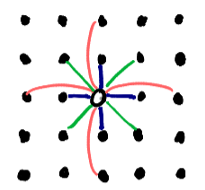 The layout of the springs is portrayed in the figure to the right. Each
dot represents neighboring particles, and the hollow dot in the center
represents the particle of interest. If the particle of interest is located at
coordinates ( i , j ) in a 2D arrangement of particles, the springs attached to it
are as follows:
The layout of the springs is portrayed in the figure to the right. Each
dot represents neighboring particles, and the hollow dot in the center
represents the particle of interest. If the particle of interest is located at
coordinates ( i , j ) in a 2D arrangement of particles, the springs attached to it
are as follows:
- stretch springs (blue): (i, j) connects to each (i+1, j), (i-1, j), (i, j+1), and (i, j-1)
- shear springs (green): (i, j) connects to each (i+1, j+1), (i-1, j+1), (i-1, j+1), and (i-1, j-1)
- bend springs (red): (i, j) connects to each (i+2, j), (i-2, j), (i, j+2), and (i, j-2)
Outside of understanding the basic structure of the system, the particles do not need to actually be referenced in a 2D manner. Only referring to the set of particles as a 1D array allows for a more generic and streamlined system. However, what does benefit from a 2D arrangement is the collection of springs connecting those particles. That is because one spring can theoretically connect to any two particles in a system. As such, the layout for the spring collection is a 2D matrix with dimensions n by n where n is equal to the total particle count. This results in a sparse matrix in which each occupied element stores the information for the spring connecting two different particles.
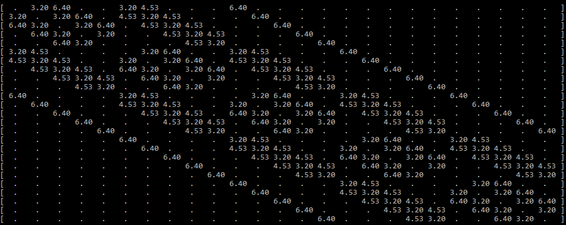
An example is seen in the figure above, which displays the sparse spring matrix for a mass-spring system with 25 particles (a 5x5 patch). To prevent clutter, the filled elements are only showing one piece of data (the rest length of the spring). There are a few key features of this sparse matrix that are important to note.
One feature is that the matrix is diagonally symmetric. This is due to the aforementioned facts that the matrix’s dimensions are the total particle count in each dimension, and that a spring connects two particles. Because of this, if one particle with the ID x is connected to another particle with the ID y , the same spring will be located at both ( x , y ) and ( y , x ).
The most important feature to note builds off of the previous feature. Every spring that connects to a particle can be found in its respective row or column. That means when calculating the spring forces for each particle, only one row (or column) needs to be accessed to find the total spring force directly affecting the particle.
However, the sparse matrix is still very wasteful to use directly in computation. With how the springs and mesh are defined, there is a maximum of 12 springs per particle, but there may be tens of thousands of particles. Meaning only 12 elements per row of tens of thousands of elements are actually needed for computation. The maximum spring count could be a bit different if a more irregular mesh was used, or if different springs (like sewing springs) were added to the calculation, but it will still be significantly less than the total number of particles, especially at the sizes considered for GPU utilization.
Considering how sparse the matrix is, it would be wise to use a sparse matrix storage system. Because of the diagonal nature of the array, the first thought may be a DIA format, but doing so would not be beneficial. The elements are fairly close to the diagonal when the particle count is low, but they spread out as the particle count increases, which is not ideal for DIA. Also accessing per diagonal would mean the calculation would result in a scatter implementation rather than a gather implementation. In order to keep the main calculation as generic as possible (allowing for any piece of cloth or pieces of cloth as long as there is some spring matrix defined for it/them), a compressed sparse row (CSR) format is used. With CSR, a single compressed row can be used per particle in the calculation of spring forces.
The main spring system is now fully defined, but there are also some extra features including colliders, external forces, and pinning. Most are either single constants or small arrays, so they are not worth being thoroughly discussed in this section.
Calculation
With the structure of the program defined and initialized, the calculation of the simulation can begin. The basis of how the calculation is performed is with explicit integration, which presumes the velocity and acceleration of the particles are constant during a time step, and those values are used to solve for the next time step. This is an intuitive and fast way to calculate the forces in a simulation but is prone to being unstable if the time step is too large. The goal fps of 30 would result in way too large of a time step, so the simulation runs several times per frame. The time step chosen for the cloth simulation is 1000Hz. Thus, the simulation runs 34 times a frame (the last time step in the frame has a shorter length to compensate for fractions of steps per frame).
In each time step, there is a loop that runs through each particle in the simulation (this loop is replaced by a kernel for the GPU implementation). So, one iteration of the loop represents the calculation for the next time step for one particle. The data for the particle of interest gets copied to a local variable (since the particle data is considered constant during the time step). The local particle ( p ) and a local variable to keep track of the total force on that particle ( f ) are the two focus variables. The calculations performed on those variables are as follows:
- Loop through the corresponding row of the CRS and calculate the spring and damping force (per element in that CRS row)
- Spring force using Hooke’s Law
- Damping force: force applied to oppose a fraction of the motion
- Add wind/gravity force vector
- Check collision with objects
- Proximity check (per object)
- If colliding, cancel out the velocity and force component in the direction of the object normal
- Check collision with the floor
- Proximity check
- If colliding, cancel out the velocity and force in the z direction
- Check collision with other particles
- Proximity check (per particle)
- If colliding, apply elastic collision
- Use the new force and velocity to find the velocity and position for the next time step and assign it to the local particle.
- Set the corresponding return array element to the updated local particle
Suitability for GPU Acceleration
For the GPU implementations, the main focus was the real-time aspect of the code. The creation of the CSR has a lot of divergences, is mostly sequential, and only runs once for a short period of time, so it would be a poor fit for converting to run on the GPU. On the other hand, everything that is done per frame (aside from launching the kernels the correct number of times per frame) can be transferred onto the GPU and stay on the GPU.
The explicit integration implementation used for this project is suitable for GPU acceleration because as long as the time step is suitably low enough, the calculation for the new particle data only needs to rely on its current data and the current data of the particles directly connected to it. Thus, the spring forces can be gathered from the connected particles and assigned to an individual particle per thread. Also, since only one particle is being written per thread, and the particle array is a 1D array that can grow rather quickly with more detailed pieces of cloth, the blocks on the GPU will be filled and occupied entirely, except for the very last block for the array.
GPU Implementations
There were a number of iterative implementations of the GPU version of the code which are all described in this section.
In the initial naive implementation, the code was mostly only changed enough to be able to run on the GPU. Each thread was assigned a particle, and it would be written to a separate but identical buffer at the end of the kernel. To prevent race conditions, the particle at the current index was copied to a register. The particle data was the only non-local data that explicitly needed this in order for the kernel to run properly, but any global data that was being read multiple times within the kernel was also copied to a register.
The next implementation was a small change to see how constants would benefit the execution. Every argument that was not being written to was given the const keyword. This was not expected to make a huge difference since the only variables able to fit in constant memory were scalar variables and the fairly small object array.
The next implementation was focused on seeing how optimizing the math during the computation could affect performance. There were a couple of small changes made, but the one expected to make the largest difference was the switch from using distance to the squared distance to determine proximity for collisions. The square root operation is expensive, so omitting it and squaring the threshold value would result in the same comparison being made.
It was unclear if this next implementation would cause a speedup, but it was worth trying. As mentioned in the calculation, there are two particle buffers being passed in: the input and the result buffers. After the kernel is done running, the result buffer is copied back to the input buffer so the next time step has the updated data for the particles. This implementation changed the CPU logic for running each kernel per time step. Rather than there being explicitly one input buffer and one result buffer, the two buffers swapped roles each time step. For example, after a single time step, the result buffer is holding the updated information while the input buffer is now outdated. For the kernel in the next time step, the result buffer is passed as the input buffer and the outdated input buffer is passed as the result buffer so the old data can be overwritten. This avoids the need to copy back the buffer but adds some CPU logic.
The next implementation was a big shift for the self-collision section of the code. Rather than checking the current particle against every other particle for a potential collision, binning was used to limit the number of comparisons to only those close to the current particle. This in and of itself changes the scaling of the problem since the speed of the self-collision is no longer directly dependent on the total particle count. In this step, the update kernel for the bins was kept naive and foolproof to ensure the binning was working properly. In the update kernel, each thread was assigned a bin and it checked against all the particles to find the particles contained inside the bin. To prevent unnecessary amounts of calculation, the update kernel could be launched only every frame rather than every time step, because the neighboring particles were unlikely to change significantly between time steps.
The next and final implementation was focused on improving the efficiency of the bin update kernel. Rather than the bin checking against all particles, only the particles in the neighboring bins (a 3x3x3 area surrounding the current bin) were considered. It is very unlikely that a particle will skip an entire bin over the course of a frame. The simulation would break before that could happen. So this is a way to significantly reduce the number of particles checked, and prevent the bin update kernel from scaling based on the total particle count.
Results
Speedup Over CPU at 25.6k particles
Performance metrics were taken with a AMD Ryzen 7 3750H and NVIDIA GTX 1660 Ti
For a more recent benchmark, the “Binned Neighbors” implementation runs at ~5 ms frame time (~200 fps) using a RTX 4070
| Technique | Speedup over CPU |
|---|---|
| CPU | 1.00x |
| Naive GPU | 108.51x |
| Constants | 110.88x |
| Math | 154.90x |
| Buffer | 154.68x |
| Binned Refresh | 156.70x |
| Binned Neighbors | 1,635.58x |
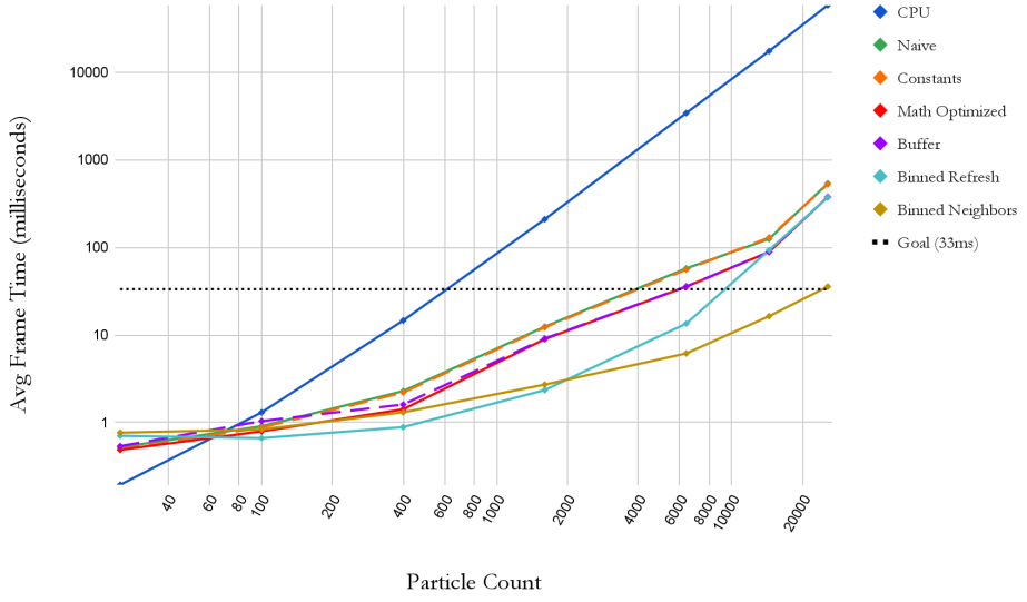
A series of different size meshes were used to test each implementation at various particle levels. The sizes 5x5, 10x10, 20x20, 40x40, 80x80, 120x120, and 160x160 result in the particle counts of 25, 100, 400, 1600, 6400, 14400, and 25600 respectively. The graph displays the averaged frame time for each implementation as the particle count increases. Log scales are being used for a clearer comparison. As expected, the CPU has better utilization at very low particle counts; meanwhile, the GPU is being underutilized for any of the implementations. However, as the particle count increases, the GPU implementations easily beat out the CPU implementations.